What are the Properties of Air? Part Two.

When it comes to air movement, understanding the properties of air is vital. In this series of articles, we look at how different parameters affect air density, and how air density changes take place within an Air Handling Unit (AHU).


Air Density

The density of air is a useful value in measuring the air volume. It is defined as the mass per unit volume of air, and its value is affected by a number of factors, including altitude (air density decreases with increasing altitude, like air pressure), and variations in temperature and humidity.

The equation for calculating air density is shown in Figure One.


Calculating Air Density

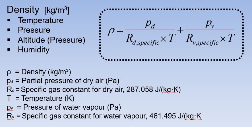Figure 1: Calculating Air Density

At sea level, at a temperature of 20°C, at International Standard Atmosphere (ISA), air has a density of approximately 1.2 kg/m3.

As we saw in Properties Of Air Part One, Relative Humidity is the ratio between the maximum water that the air can hold (100%) and the actual water content at the current temperature. It can also be expressed as the ratio (in per cent) of the vapour partial pressure of the air to the saturation vapour partial pressure at the actual dry bulb temperature, or by the actual mass of the vapour and the air.

The biggest environmental factor which will affect air density is temperature: a change of just 6°C (from 20°C to 26°C will change the density by 1.7%. Pressure has a smaller but still tangible impact: a 500Pa change in pressure will change the density by 0.49%. The effect of changes in humidity are almost negligible: a large change of 25% in humidity will only change the air density by 0.37%.

The Mollier Chart

The Mollier Chart was devised in 1904 by Richard Mollier in Dresden. It is an enthalpy-entropy chart, describing the enthalpy of a thermodynamic system.

The Mollier Chart is used in order to design air conditioning processes and to calculate, among other things, the change in temperature and humidity, and the energy required to heat or cool the air. In FläktGroup's product selection software ACON, a Mollier Chart with the specific air handling unit process can be plotted automatically.

Figure Two shows a typical Mollier Chart.

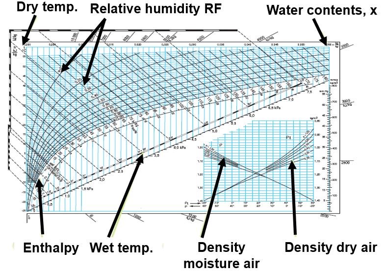Figure 2: A typical Mollier Chart

Calculation Of Air In An Air Handling Unit

Figure Three shows a typical Air Handling Unit, showing eight positions air must pass through, each of which will change the air on its journey from ambient air (position #1) to the desired air condition (position #8).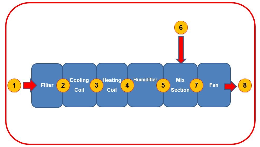


Figure 3: The eight positions of a typical Air Handling Unit

Let’s take an example. Suppose the outdoor condition (position #1) is a temperature of 27°C with 65% relative humidity. We are at sea level, with an atmospheric pressure of 1013 mbar – a typical summer’s day. The requested supply air condition (position #8) is a temperature of 22°C, with a humidity of 40%, an airflow of 6m3/s, and a 500Pa available pressure to compensate for the pressure drop in the duct system.

The first calculation is to find out the air density of the outdoor condition. Using the Ideal Gas Law shown in Figure One, the calculation looks like this: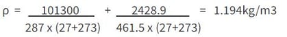




Position #2

Once the air has passed the filter, the temperature, density and humidity will stay the same. The under pressure will have increased to compensate for the filter pressure drop (in this case -85Pa).

Position #3

Now we come to the cooling coil. In this case we want to use it to reduce the humidity in the air, which needs the temperature to be lowered below the saturation point. Calculating the cooling power at this stage uses the formulae outlined in Properties Of Air Part One. Using the enthalpy formula will give us the total power needed, including both sensible and latent power; using the temperature as a parameter will give us the sensible power on its own, as follows:


Ptot = 5 x 1.2 x 1.01 x (64-20) = 266kW
Psens = 5 x 1.2 x 1.01 x (27-8) = 115kW


With a 100Pa pressure drop through the coil, the cumulative pressure drop is now -185Pa.

After passing through the cooling coil, the temperature is 8°C and the humidity 100% (because the saturation point has been passed). This means that the air density is higher; using the same calculation as before, it is now 1.26kg/m3.

Position #4

Once the air has been dehumidified, the heating coil will increase the temperature. It doesn’t matter if you use the enthalpy or temperature formula for calculating the power, as with no change in state (and hence no latent power required), the result will be the same:

Ptot = 5 x 1.2 x 1.01 x (20-8) = 73kW

With a further 50Pa pressure drop in the heating coil, the cumulative pressure drop is now -235Pa. the density is now 1.217kg/m3.

Position #5

In this case, the humidifier is not necessary to reach our goal of 6m3/s airflow and 40% relative humidity.

Two things provide humidity to the air. The first is condensation, by spraying water over a ‘block’ that the air is passing. This will lower the air temperature, which has to be compensated in the AHU with heating if necessary.

The second method is providing steam into the air with lances in the AHU. This will only change the humidity in the air, and has no effect on temperature – and gives a very low pressure drop.

Combined Effect Of Positions #5, #6 and #7

In our example, two airflows are mixed, from the inlet (position #5) and from recirculation (position #6). To calculate the condition of this mixed air, there are two methods.

The first is to use the Mollier Chart; draw a straight line between the two points of airflow, then measure the distance between those points on the line that has the same ratio as t he two airflows – that point is the new condition (point 8(7) in Figure Four). You can then use the chart to read the temperature and humidity.

Alternatively, you can use the theoretical method. Assuming the airflow from the inlet is 5m3/s at 20°C and a 35% humidity, and the airflow from recirculation is 1m3/s at 25°C and 50% relative humidity, then by multiplying the ratio between the airflow by the temperature difference, and then adding to the lower temperature of 20°C, will give you the new temperature:

(1/6 x (25-20)) + 20 = 21°C

The total airflow is a simple addition of the two airflows (so 5m3/s + 1m3/s = 6m3/s). You can read off the humidity at the new point on the Mollier Chart.

Position #8

Having passed through the entire AHU, our goals has been reached. Note that the fan will increase the temperature by up to 1°C, depending on the size and workings of the motor. In this case we have assumed it raises the air temperature by 1°C, giving us our desired temperature of 22°C.


Figure Four shows the complete Mollier Chart for our example, plotting all eight positions.

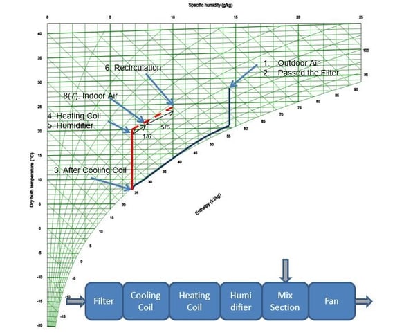
Figure 4: Mollier Chart plotting changes in air in the example given

Recalculating Density

The air density as the air passes through the AHU varies, with the most significant effect occurring when changing temperature. At each stage the density can be calculated using the Ideal Gas Law shown in Figure One.

When testing an AHU, and to compare the result with other units or the catalogue values, it is important that you can recalculate to standard density. The two properties which will be changed when they are recalculated to standard density are airflow and pressure. This means you have two ways of recalculating: leaving the airflow constant and changing the pressure by multiplying with the density ratio will give you the new pressure at the same airflow: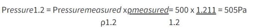



AHU: 6m3/s at 505Pa


Alternatively, you can leave the pressure constant, giving you the new airflow at standard density: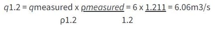



AHU: 6.06m3/s at 500Pa

Missed Part One?

Read it here: What are the Properties of Air? Part One.